Physical Site Optimization

Physical Site Location is an interesting Analytics problem that many face: from Grocery Stores to Telcom and Apparel Retailers ...  One may run BI (Find Look-alike stores, Find performance Headroom) or play an Expansion scenario (Find best location for a next store).  

However, some problems do not fit into a boilerplate solution and require some ad-hoc analysis. Today, I will talk about a little simulation I ran that looks at 2 non-conventional scenarios.

Background:

Let's assume that the client is a major maintenance provider that has decided to enter the French Market to service 2,000 "client sites" and commissioned your company to optimize the location of its sites with 2 scenarios:

1- Organic: Starting from scratch, which locations are best at optimizing the travel distance to the client sites? How many maintenance sites are required and what would be the workload of each?

2- Acquisition: Given the existing site network of a potential acquisition target, how many sites of those existing sites, need to be upgraded to service the customer base. The client initial solution was 30 out of the 131 sites.

To spice up scenario 2, we also add a service (SLA) constraint of a 120min maximum driving time.

Scenario 1:

Here is the process I followed:
1- [R]: Calculate all possible travel distances using great circle distances (note that for short distances like France has, an easy Cartesian approximation is also possible)
2- [R]: Run a k-means clustering on the client sites for several k = 2...40 (number of clusters)
3- [Tableau]: Analyze the distribution of clients and the workload associated to each of them

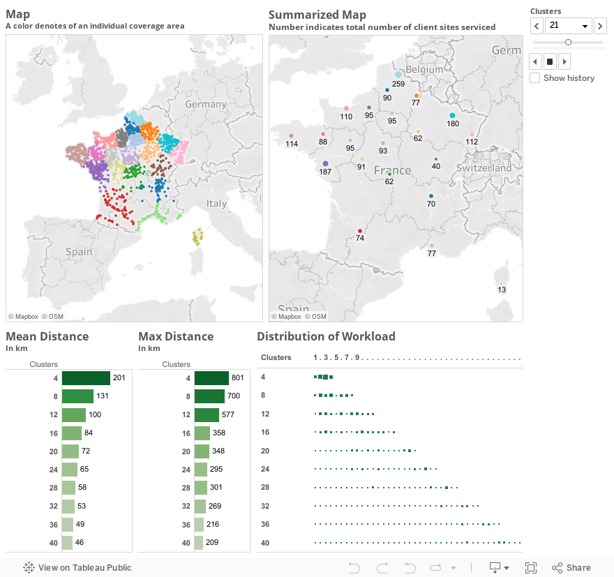
In this scenario, we get a quick understanding of the meshing of the national territory as the Tableau below demonstrates:

Learn About Tableau

It looks like the client sites are heavily located in Brittany and Northern France. Overall, less than 20% of the sites are located South of Poitiers (i.e. bottom half).

Let's take an example, with 16 sites, a client would be located on average at 100km and a maximum distance of 358km (probably due to low coverage in the South West)! As we can see, the clustering focuses on minimizing the average travel distance and, as a consequence, sites on the frontier can be challenging to service within a SLA.

You can also "play a story" - a nice feature of Tableau - by increasing k iteratively. Note that the action mostly happens in the North (consistent with the center of gravity).

Future Considerations:

Note that for insular locations, it would make sense to manually force the clustering algorithm to set them aside by assigning them far-away locations (say Africa for instance). That way, it will naturally make a cluster out of those instances on the first k (that's because k-means is sensitive to outliers).

In addition, this simplistic method doesn't take into account the quality of the roads, speed limits and other influencing variables but it something that can be done afterward, to determine the location of the Maintenance Centers (within each cluster). In others words, it gives out a natural meshing of the territory that can be refined as a second step. In scenario 2, we will see how to integrate that information.

Scenario 2:

Scenario 2 is slightly more complex and the initial thought was to use brute force. For instance, if looking at 40 sites among 131, I would look at all combinations which leads to ... 7.67 E+33 ... That will not work well. My next move (and the one I adopted in this scenario) was to use a, sometimes overlooked, algorithm from my Operations toolbox: Linear Optimization. 

Let's look at the following steps: 

1-  [R] Collecting Driving Distance  

Fetch the actual driving time for all combinations (Maintenance Center X Client Site) requires using an API (Google Distance API works well but is limited in terms of calls). I decided to chose MapQuest API. To that end, I created a little R wrapper that uses the MapQuest API "Distance Matrix" functionality.(module: Time for Many to One). For each selected combination (Maintenance Site X Client Site), it returns the driving time at the current time of the day and in current driving conditions (do not run it at night if the services are to occur at traffic jam time).

In order to reduce the complexity of the problem, we can only make calls to the API for combinations (Maintenance Site X Client Site) are that on the fence:





I chose the frontier to be [80km - 120km]. Under this hypothesis, anything below can be serviced within 120min, anything above won't.  This reduces the number of combinations to check by  97% without impairing the results.  Of course, expanding the frontier area would give you more accurate results.

The result of this step is a Travel Time Matrix of shape (Number of Maintenance Sites X Number of Client Sites), each cell representing if a given Maintenance Site can service a Client Site.

2- [R] Running Linear Optimization: 

This problem is essentially about minimizing the number of sites under a constraint (the SLA). As such, it perfectly fits in a linear programming framework and it can be written as follows:

• Minimize the number of sites (denoted f.obj below)

• Under the constraint that at least 1 site is within the predefined driving distance (f.con)

In R, it translates into this:

 lp_object <- lp("min", objective.in= f.obj,   
          const.mat=f.con, const.dir= f.dir, const.rhs= f.rhs,   
          all.bin=T)  

all.bin=T means that a site can either be upgraded or not.

The algorithm that runs under-the-hood is a discrete optimization named Branch-and-Bound and ensures of a global minimum, if any. 

Before starting the optimization, it's safer to check you have a solution (at least 1 maintenance site is within driving distance for each client site). Otherwise, it won't converge.

The little cherry on the cake: it is also very fast.

3- [Tableau]: Visualization: Now we can look at the results interactively with Tableau in order to:

• Validate the results (does the distribution of maintenance sites make sense visually?) - At this point, a human can clearly see if the selection covers the territory properly

• Play several scenarios on the distance requirement parameter (see if a SLA relaxation improves considerably the savings - which may lead the business to renegotiate terms before launch)

• Quantify the savings

Here is what it would look like:

Learn About Tableau

The numbers look quite compelling with savings north of Eur 1MM thanks to finding a good solution with only 27 maintenance sites (vs. 30 that the client estimated).

Note that by loosening the drive time requirement to 150min , the savings would be also Eur 5MM with only 17 sites ! Locations like Corsica would save 1 maintenance site (from 2), quite a good opportunity to explore as a lead for further savings.

Conclusion:

Site optimization is a fun Analytics problem (and a good excuse to make nice maps!). Usually, it can be solved with a combination of R + Tableau since the data is relatively small. 

Like in any Analytics problem, visualization is super-important as it conveys the results of your analysis. A nice, interactive and user-friendly Tableau is worth more than a long explanation.

In my experience, it's useful to simplify the problem as much as possible from the get-go. For instance, many combinations (Maintenance Sites X Client Sites) are visibly improbable thus can be removed from the equation. 

I share my code. Feel free to request it to me.